|
| Figure 1. An idealised representation of the interplanetary medium between the Sun and the Earth (adapted from Smart [1988]). |
| Table of Contents | ECSS | Model Page |
| Background Information | Background Information | |
| Solar particle models | ||
A number of significant events associated with past solar cycles may have been responsible for several spacecraft operational anomalies. Furthermore, radiation protection is a prime issue for space station operatons, for extended missions to the planet Mars, or for a return visit to the Moon. For these reasons and others, considerable interest has been shown in recent years concerning the prediction of solar proton fluences from data collected during past solar cycles.
The trend in recent years towards smaller and faster electronic components and more sensitive detectors has resulted in a need to understand and protect against solar proton effects on spacecraft systems. In earlier satellites, larger components were used which meant that single particles could only affect a limited volume of the device, and thus only cumulative damage resulting from multiple particle interactions could lead to malfunction. With the size of modern devices minimised to improve processing speed and power consumption, a single particle can have a significant effect and even cause irreversible damage to an electronic device. As a consequence, these devices are more susceptible to radiation effects than older components.
The main mechanism which allows an energetic proton to deposit energy as it passes through matter is ionisation. The energy given up by the incident particle results in the formation of electron-hole pairs which in turn causes the device performance to degrade.
Displacement damage occurs when the incoming energetic proton transfers momentum to atoms of the target material. If sufficient energy is transferred, the atom can be ejected from its location, leaving a vacancy or defect. The ensuing physical processes are varied and complex, but once again reduced device performance is the ultimate consequence. This is an important mechanism in solar cell, CCD, opto-coupler and material degradation.
Two further mechanisms of importance are those of the single event upset (SEU) and the single event latch-up (SEL) which occur when an incident charged particle deposits a short but intense charge trail in the sensitive volume of a component. This charge trail is capable of reversing the logic state of a memory element (SEU) or causing destructive latch-up where a parasitic current path is created, allowing large currents to destroy the device. This process is mainly limited to ions of higher atomic number than protons, since the linear energy transfer (LET or dE/dx) of heavy ions is significantly greater than that of protons. However, energetic protons can undergo nuclear interactions with component materials and the short range reaction products lead to an intense local charge generation, producing an SEU or even a latch-up.
Solar cell performance is also adversely affected by the ionisation and displacement mechanisms described above. Degradation results in the reduction of both the voltage and current output, which may have severe implications for the spacecraft lifetime.
Solar cells are usually made of silicon, although gallium arsenide cells can provide enhanced efficiency at increased production cost. They are arranged in series and in parallel to provide desired voltage and current levels, respectively, and collectively form the solar array. Thus, if a single cell fails in a string of cells, an open circuit will develop resulting in total power loss. Solar cell strings can be arranged in such a way as to minimise power loss from a complete array, but degradation is inevitable.
Solar cells are protected at the front by coverglass, providing shielding against protons. Annealing processes can also offset performance degradation caused by the ambient radiation environment. This is especially true for gallium arsenide cells and to a lesser extent for silicon cells.
Future interplanetary manned missions will need to consider solar flare activity very carefully due to the obvious detrimental effects of radiation on man. Very high doses during the transit phase of a mission can result in radiation sickness or even death. This is equally true for extended visits to surfaces of other planets and moons lacking a strong magnetic field capable of deflecting solar particles. The risk of developing cancer several years after a mission is somewhat more difficult to quantify, but must also be considered in mission planning.
Adequate radiation protection measures must be conceived for any lengthy interplanetary endeavours. Storm shelters will be necessary both on the transit spacecraft and on the planet surface. The latter can be provided to a certain extent by geological features of the visited body. The design of radiation shielding for a spacecraft is much more difficult given the inherent limitations associated with the construction of an interplanetary space vehicle.
SPENVIS Provides access to the following radiation effects models:
Short term forecasts are necessary for any tasks requiring extravehicular activity (EVA) and the operation of radiation sensitive scientific detectors. Real time observation of the Sun can provide useful warning of solar flare activity, as large proton events are usually associated with the strong emission of electromagnetic radiation, such as visible light, radio waves and soft X-rays during a flare.
By virtue of travelling at the speed of light, electromagnetic radiation reaches the vicinity of the Earth (or any other location in space) before any particulate radiation arrives (it takes electromagnetic radiation 8.5 minutes to reach the Earth from the Sun, whereas non-relativistic particles reach the Earth only hours or days later, depending on the particle energy). Protons first need to propagate through the solar corona to the foot of an interplanetary magnetic field line by diffusion. This process can already cause significant attenuation of particle fluxes if the flare site is a great distance from the field line. The next step is propagation through the interplanetary medium along the magnetic field lines, which during quiet conditions adopt an Archimedean spiral configuration. During this stage of propagation, the solar proton population can be significantly modified by several physical processes such as diffusion and acceleration caused, for example, by interplanetary travelling shocks or corotating interaction regions. Protons are usually scattered by the interplanetary medium, resulting in quasi-isotropic fluxes. However, certain large scale features of the magnetic field such as magnetic bottles or clouds can cause charged particles to temporarily adopt highly anisotropic distributions.
The most direct interplanetary field line connection with the Earth originates close to a heliographic longitude of 60° west. Thus it is quite possible that a large flare sited well away from this longitude will produce an insignificant increase of solar proton fluxes at the Earth. It is therefore important to be able to distinguish such false alarms which would otherwise interfere with spacecraft operations for no valid reason. Equally essential is to be able to obtain prior warning of solar protons when no electromagnetic activity has been monitored. This can happen when the flare site is hidden behind the solar limb, thus making optical, radio or X-ray observations difficult, if not impossible. An idealised sketch of the interplanetary medium and the propagation of radiation between the Sun and the Earth is shown in Fig. 1.
|
|
| Figure 1. An idealised representation of the interplanetary medium between the Sun and the Earth (adapted from Smart [1988]). |
Long term predictions of the radiation levels resulting from events are required if costly overdesign or mission threatening underdesign are to be avoided. The dose accumulated over a mission lifetime is a function of the solar proton fluence (except for low inclination low Earth orbits, where geomagnetic shielding provides protection), so a reliable estimate of this fluence is needed by a spacecraft engineer to optimise design parameters.
As with any form of long term forecasting based on past observations, the statistical interpretation of data plays a central role in the final model definition. The size of the data set used will always be a limiting factor to the level of confidence associated with any solar proton model. In situ measurements of solar event particles by satellites have only been available since the early days of the space age. Prior to that, solar event fluences could only be inferred through ground based or low altitude measurements made by sounding rockets or balloons. Unfortunately, such techniques are prone to inaccuracy and can only be used with any real confidence for the last solar cycle before the advent of satellite technology.
|
| Figure 2. Annual mean sunspot number. The blue and green vertical lines indicate the dates of solar maximum and minimum, respectively; the red rectangles show the solar maximum periods defined by Feynman et al. [1993] for the JPL models. |
Predictions for solar cycle 21 indicated that the sunspot number would most probably be less than that measured during cycle 20, although this turned out to be false. Assuming that sunspot number and annual integrated solar proton fluence were linearly related, King chose to ignore the solar cycle 19 data set and took measurements made only in cycle 20 as representative of cycle 21.
The data set was mainly constructed from proton measurements (in the energy range 10-100 MeV) made by instruments on IMP 4, 5 and 6, which all flew in geocentric, highly elliptic orbits. The data from any individual instrument or satellite were cross-calibrated with independent measurements whenever possible, to check the mutual consistency of the complete data base.
There are 25 individual events used in the King data base, including the great proton event of August 1972, which accounted for about 70% of the total >10 MeV fluence for the complete solar cycle. Since this large event made such a dominant contribution to the total solar cycle fluence, King decided to separate it from the remaining 24 events, and to class it as an anomalously large (AL) event, in contrast to the remaining ordinary events. It is commonly accepted that if an Apollo mission had flown during the August 1972 event, the astronauts would have received severe (and potentially lethal) doses of radiation. Apollo 16 flew in April 1972 and the following (and final) mission of the programme flew in December of the same year.
The statistical approach used by King was based on methods employed by Yucker
[1972] and Burrell [1972] in their analyses of earlier solar proton data.
Yucker introduced the concept of compound probability to define the probability
P of exceeding a specified fluence f of protons with energy
greater than E during a mission lasting t years as

The integrated energy spectrum of the August 1972 event was found to be best
represented analytically by an exponential in energy:
|
| Figure 3. Spectra used for the King [1974] solar proton model: ___ AL event spectrum; ___ mean ordinary event; ___ 90% worst case ordinary event. |
The data set used by Feynman et al. [1990] for the first version of the JPL model (JPL-85) includes observations obtained between 1956 and 1963 (during solar cycle 19) using detectors flown on rockets and balloons. After 1963, satellite monitoring of the near-Earth radiation environment became routine and an essentially continuous data base has been collected from measurements made by several spacecraft. The data used for the JPL-85 model cover three solar cycles.
Using the exact dates of solar maximum (1957.9, 1968.9, 1979.9 and 1989.9) as the zero reference year for each cycle, Feynman and colleagues were able to demonstrate that the active phase of the solar cycle lasted for 7 years of the complete 11 year cycle. The years of high fluence begin 2.5 years prior to the zero reference date, and end 4.5 years after this date (see Fig. 2). An asymmetry in the event frequency and intensity therefore exists with respect to the peak in solar activity. The JPL model only considers solar proton fluences throughout the seven hazardous years of a solar cycle, and ignores fluences during the remaining four quiet years.
The JPL-85 model has been replaced by a newer version, JPL-91 [Feynman et al., 1993]. The occurrence frequeny of the major events that dominate the total fluence do not appear to be randomly distributed in time. Instead, they appear to be much more common in some solar cycles than in others. In particular, in the 25 years between 1963 and 1988 there was only one major event (1972). In contrast, 3 or 4 major events occurred in the short time period from 1957 to 1963, and 4 or 5 major events have occurred between 1989 and 1991. It is therefore essential that the data set for a solar proton model is collected over several solar cycles so that it contains a good statistical sample of the major events. At the time the JPL-85 model was constructed, only one major proton event had taken place since 1963 when data collection in space had become routine. In the JPL-85 model this problem was dealt with by using data that had been collected before 1963. Although these data were of surprisingly good quality, they were collected and analysed with different techniques from the data collected after 1963. For that reason, the data set used in the JPL-85 model did not form a uniform data set. The occurrence of major proton events in the early nineties provided the opportunity to correct this weakness of the JPL-85 model. At the same time, the model energy range was extended.
The data set used for the JPL-91 model consists of a nearly continuous record of daily average fluxes above the energy thresholds of 1, 4, 10, 30, and 60 MeV. The proton events considered in the JPL models are defined as the total fluence occurring over series of days during which the proton fluence exceeded a selected threshold. The thresholds for the JPL-91 model (in cm-2 s-1 sr-1) are 10, 5, 1, 1, and 1 for the five energy thresholds.
The statistical properties of the events occurring during active periods of the solar cycle are considered separately from those occurring during the quiet periods. For the JPL models, it was assumed that no significant proton fluence exists during quiet periods and that the only model needed is one for the active periods. Therefore, only data collected during the 7 active years of the cycles were used.
The cumulative probability distribution of the high fluence portion of the data can be fit quite well with a lognormal distribution. Figure 4 shows the distribution of the solar event fluences for protons of energy >60 MeV. The events have been ordered according to the log of the fluence and plotted versus the percent of observed events that have a magnitude less than the given event. The horizontal axis of the plot is scaled so that a data set that is distributed lognormally will appear as a straight line. The real distribution of the data is not lognormal since in the real data there are always more events the smaller the size of the event, whereas for a lognormal distribution there is a mean event size and the number of events decreases for events both smaller and larger than that mean. For this reason, the distributions cannot be expected to be fit by a straight line for fluences less than the average of the data set. However, the estimate of the total fluence accumulated during a mission is dominated by the estimate of the probability occurrence for large events and will not be changed due to the underestimate of the probability of occurrence of the small events. The important question is the estimate of occurrence of the largest events. The straight line fit to the event fluence distribution is superimposed in Fig. 4.
|
| Figure 4. Distribution of solar event fluences for solar active years between 1963 and 1991 for protons of energy >60 MeV for which daily averaged flux exceeds 1.0 cm-2 s-1 sr-1. The straight line is the fitted lognormal distribution (from [Feynman et al., 1993]). |
The formulation of the JPL models is exactly the same as that used by King with
the exception of the definition of the function
p(n,t;N,T). The JPL data set has a
significantly larger population of events so that pure Poisson statistics are
applicable:
The JPL models are presented as probability curves of exceeding a given fluence during a mission of a selected duration. The fluence probability curves for various misison durations are represented in Fig. 5 for protons of energy >60 MeV. The probability curves give the probability of exceeding a given fluence during the life of the mission assuming a constant heliocentric distance of 1 AU. To use the probability curves, find the line that corresponds to the desired mission length during solar active years (the fluence in a single 11 year cycle should be assumed to be equal to 7 year fluence). Locate the confidence level required, recalling that a confidence level of say 95% means that only 5% of missions identical to the one considered will have fluences larger than that determined for the 95% confidence level (i.e., probability + confidence level = 100%). Then, the abscissa gives the fluence that will not be exceeded with the selected confidence level. In the numerical implementation of the models, the probability curves are represented as a discrete set of points between which linear interpolation is performed. Interpolation or extrapolation for energies different from the model thresholds uses an exponential fit of the fluence in terms of rigidity.
|
| Figure 5. Fluence probability curves for protons of energy >60 MeV for various mission durations (from [Feynman et al., 1993]). |
Feynman et al. [2002] have studied the observations of solar particle events that have occurred since the JPL 1991 model was developed (up to 1998) and concluded that the new observations fall well within the distribution of fluences upon which the JPL 1991 model was based. Hence, the authors conclude that no change need be made to the probability distribution used in the JPL 1991 model and that it is no longer necessary to label the JPL model by the year during which the data set terminated. The model can now be called simply the JPL model.
| Parameter | >10 MeV | >30 MeV |
|---|---|---|
| log10(μ) | 8.07 | 7.42 |
| log10(σ) | 1.10 | 1.2 |
| w | 6.15 | 5.40 |
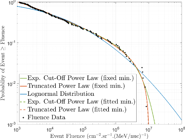
Previous approaches to modelling solar proton event fluence distributions have been largely empirical in nature. Lognormal distributions have been used to describe large event fluences, but deviate from the measured distributions for smaller event fluences [King, 1974; Feynman et al., 1993]. Power laws, which describe the smaller event fluences very well, but overestimate the probability of large events, have also been used [Gabriel and Feynman, 1996]. Both of these types of approaches have merit. However, they do not accurately describe the complete distribution, allow for the possibility of infinitely large events, and lack strong physical and mathematical justification.
The basic difficulty in describing a solar proton event fluence distribution arises from the incomplete nature of the data, especially for large fluence events. For example, in the last 3 complete cycles, which span approximately 33 years, only 3 separate events have produced a >10 MeV fluence of approximately 1010 cm-2 or greater. Characterising the probabilistic nature of these very large events is critical for radiation effects applications.
Another reason for reassessing the cumulative solar proton event fluence models is that an accurate approach has emerged for describing the underlying or initial distribution of solar proton event fluences [Xapsos et al., 1999]. It is based on maximum entropy theory [Kapur, 1989] and predicts an initial distribution that is a truncated power law in the event fluence. The maximum entropy principle provides a mathematical procedure for generating or selecting a probability distribution when the data are incomplete. It states that the distribution which should be used is the one that maximises the entropy, a measure of uncertainty, subject to constraints imposed by available information. Such a choice results in the least biased distribution in the face of missing information. An example is shown in Fig. 6, which is a plot of the number of events per solar active year that exceed a given event fluence vs. fluence. The points represent the measured >30 MeV event fluences during active years of solar cycles 20-22. These are compared to the distribution predicted by the maximum entropy technique, shown by the line. This approach is a significant improvement in describing the distribution of events compared to previous empirical methods such as those using lognormal distributions and power laws. Since a model of cumulative fluences must be based on some initial distribution of event fluences, it is worthwhile to use the improved distribution obtained from the maximum entropy approach.
|
| Figure 6. Distribution of >30 MeV solar proton event fluences. |
Solar proton event data from the last 3 complete solar cycles (20-22) were processed to obtain the event fluences. The source of the data for cycle 20 was the IMP-3, -4, -5, -7 and -8 satellites. The data from cycle 21 was from IMP-8. The GOES-5, -6 and -7 satellite data, which extends to much higher proton energies, was used for cycle 22. Only events having some minimum fluence Φmin were considered. This minimum fluence depends on the proton energy range [Xapsos et al., 1999] and is listed in Table 1. In identifying events, the practice of NOAA was followed, where the beginning and end of an event are identified by a threshold proton flux so that a large event may consist of several successive rises and falls in flux. Since a very large portion of the accumulated fluence occurs during solar active years, it is reasonable to neglect the solar inactive years, following the practice of Feynman et al., [1993].
| Proton energy range (MeV) |
Minimum event fluence Φmin (cm-2) |
Worst case event maximum fluence Φmax (cm-2) |
|---|---|---|
| >1 | 5.0x10⁸ | 1.55x10¹¹ |
| >3 | 1.0x10⁸ | 8.71x10¹⁰ |
| >5 | 1.0x10⁸ | 6.46x10¹⁰ |
| >7 | 2.5x10⁷ | 4.79x10¹⁰ |
| >10 | 2.5x10⁷ | 3.47x10¹⁰ |
| >15 | 1.0x10⁷ | 2.45x10¹⁰ |
| >20 | 1.0x10⁷ | 1.95x10¹⁰ |
| >25 | 3.0x10⁶ | 1.55x10¹⁰ |
| >30 | 3.0x10⁶ | 1.32x10¹⁰ |
| >35 | 3.0x10⁶ | 1.17x10¹⁰ |
| >40 | 1.0x10⁶ | 8.91x10⁹ |
| >45 | 1.0x10⁶ | 7.94x10⁹ |
| >50 | 3.0x10⁵ | 6.03x10⁹ |
| >55 | 3.0x10⁵ | 5.01x10⁹ |
| >60 | 3.0x10⁵ | 4.37x10⁹ |
| >70 | 1.0x10⁵ | 3.09x10⁹ |
| >80 | 1.0x10⁵ | 2.29x10⁹ |
| >90 | 1.0x10⁵ | 1.74x10⁹ |
| >100 | 1.0x10⁵ | 1.41x10⁹ |
As discussed above, the maximum entropy principle provides a mathematical
basis for selecting a probability distribution for an incomplete set of
data. For a continuous random variable M having a probability
density p(M), the entropy S is defined as:
Regression fits to the above equation for N were performed for solar proton event fluence distributions with threshold energies ranging from >1 MeV to >100 MeV, with adjustable parameters Ntot, b and Φmax. A typical example of the fitted results is shown in Fig. 6 for >30 MeV protons. The figure shows N as a function of event fluence Φ: data is shown by the points, and the solid line is the best fit to the above equation for N. It is seen that the model describes the data well over its full 3.5 orders of magnitude. The fitted parameters are Ntot=4.41 events per active year, b=0.36 and Φmax=1.32x1010 cm-2. It is interesting to note that the index obtained here for the truncated power law is close to the value of 0.40 reported by Gabriel and Feynman [1996] for an ordinary power law. Whether or not this distribution should be truncated should ultimately be determined by the data. It is seen in the figure that the measured event frequencies begin to tail off noticeably above about 109 cm-2, thus supporting the truncated distribution obtained with the maximum entropy principle. The maximum event fluence parameter Φmax is about 1.5 times the largest observed >30 MeV fluence up to 1999. Generally, this parameter was within a factor of 2 of the largest event fluence in solar cycles 20-22.
Knowing the initial distribution of solar proton event fluences, the
worst case event can be determined as a function of confidence level and
mission duration. Assuming that the occurrence of solar proton events is
a Poisson process, it can be shown from extreme value theory [Xapsos
et al., 1998] that a cumulative, worst case distribution for T
solar active years is given by:
The upper limits on solar proton event fluences are fitted parameters that are derived from limited data. By its very nature, there must be some amount of uncertainty associated with this parameter. Thus, it should not be interpreted as an absolute upper limit. A reasonable interpretation for the upper limit fluence parameter is that it is the best value that can be determined for the largest possible event fluence, given limited data. It is not an absolute upper limit but is a practical and objectively determined guideline for use in limiting design costs.
|
| Figure 7. Probability that the worst case solar proton event fluence encountered during a mission exceeds the value shown on the abscissa with 1, 3, 5 and 10 solar active year periods. The probability of exceeding the design limit of 1.32x1010 cm-2, shown as a vertical line, is essentially zero. |
The basic SAPPHIRE provides the following set of model outputs:
SAPPHIRE is developed through ESA's (Solar Energetic Particle Environment Modelling (SEPEM) application server [Crosby et al., 2015] which is available at: sepem.eu. The SAPPHIRE model is based on data from the SEPEM Reference Data Set (RDS) v2.1 which is available here on the SEPEM server: http://sepem.eu/help/SEPEM_RDS_v2-01.zip The RDS uses as its basis data from the energetic particle sensor (EPS) on-board the National Oceanographic and Atmospheric Administration (NOAA) Geostationary Operational Environmental Satellite (GOES) series and similar instruments on-board the earlier NASA Synchronous Meteorological Satellite (SMS) series. These data have been cross-calibrated with science-class data from the Goddard medium energy (GME) instrument on-board NASA's Interplanetary Monitoring Platform (IMP-8) following the algorithms detailed by [Sandberg et al., 2014]. The result is a contiguous data set spanning over $gt;40 years (from 1974-2016) built using a fully consistent processing chain.
The Reference Event List (REL) defines SPEs by requiring that the differential flux value in the 7.38-10.4 MeV channel is above 0.01 dpfu (dpfu = differential particle flux units = particles. cm-2.sr-1.s-1.MeV/nuc-1), the minimum peak flux over the period is at least 0.5 dpfu, a dwell time of no more than 24 hours is permitted between consecutive enhancements (else they are treated as a continuation of the same SPE) and events must have a duration of at least 24 hours. The version of the REL applied in SAPPHIRE v1.0 includes 266 SPEs from between 1974 and 2016 with of the 237 SPEs occurring during solar maximum periods and the remaining 29 SPEs occurred during solar minimum.
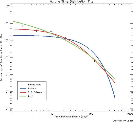
SAPPHIRE deploys the virtual timelines methodology which generates interspersed
waiting times (between SPEs) and SPE fluxes with durations based on numerical regression.
This is analogous to the monte-carlo procedure of the JPL model with the additional
consideration of the non-negligible duration of SPEs. The waiting time distribution
for solar maximum is based on a Lèvy distribution previously applied to
solar flares [Lepreti et al., 2001] and later to SPEs [Jiggens and Gabriel, 2009].
Due to the limited number of SPEs at solar minimum the time-dependent Poisson distribution
[Wheatland, 2000, 2003] was applied to waiting times for these conditions.
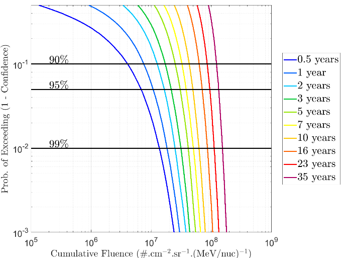
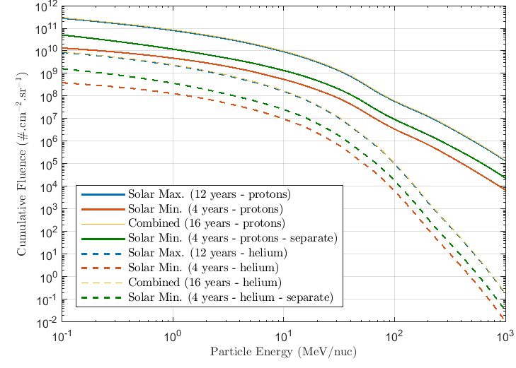
A total of 100,000 virtual timelines are used for each model result at each energy with an output
of probability of exceeding (1- confidence level) as a function of flux. The figure below shows
the proton mission cumulative fluence output for the energy channel from 31.62–45.73 MeV
for solar maximum conditions for a range of prediction periods (mission durations).
| SPE frequency (years) | Prediction period (years) | Confidence level (%) |
|---|---|---|
| 10 | 2 | 73 |
| 20 | 3 | 79 |
| 50 | 3 | 91 |
| 100 | 6 | 91 |
| 300 | 18 | 91 |
| 1000 | 26 | 96 |
| 10000 | 32 | 99.5 |
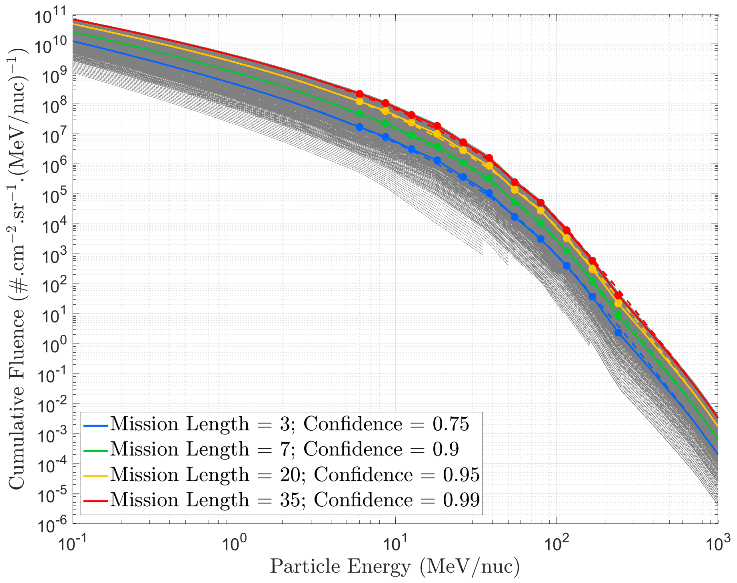
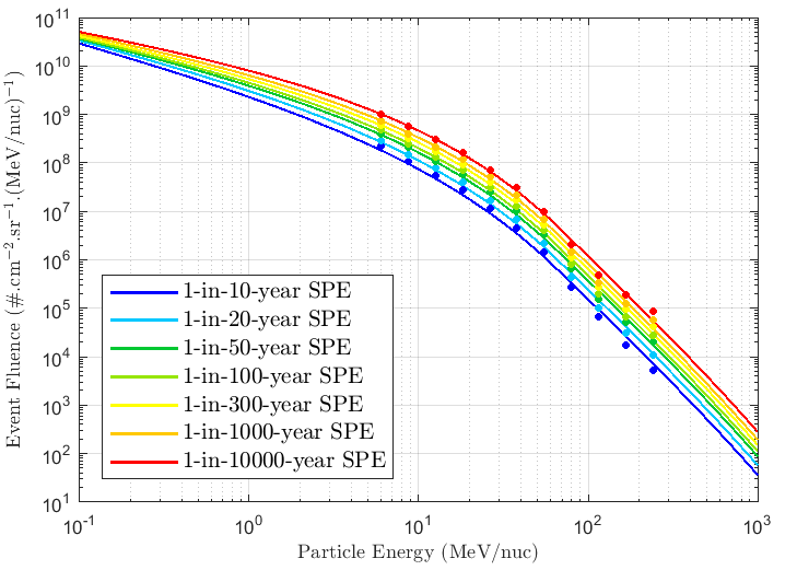
The extrapolated outputs for the SAPPHIRE 1-in-x-year SPE fluences as a function of energy are shown below:
Alternatively, the King model can be used by specifying a confidence level. With Burrell's extension of Poisson statistics, the number of events that will occur over the mission duration can be calculated, and hence the minimum number of events that need to be included. The total event fluence is then obtained by multiplying the AL or OR spectra by the number of predicted events (if only one OR event is predicted for a confidence level of 90% or higher, the 90% worst case spectrum is used). Table 3 contains the probabilities for occurrence of anomalously large events for selected mission durations.
| Mission duration t (years) | ||||
| Number of events n | 1 | 3 | 5 | 7 |
| 0 | 76.56 | 49.00 | 34.03 | 25.00 |
| 1 | 95.70 | 78.40 | 62.38 | 50.00 |
| 2 | 99.29 | 91.63 | 80.11 | 68.75 |
| 3 | 99.89 | 96.92 | 89.95 | 81.25 |
| 4 | 99.98 | 98.91 | 95.08 | 89.06 |
| 5 | 99.99 | 99.62 | 97.65 | 93.75 |
Thus, if a confidence level of 90% is required for a space mission lasting 3 years during solar maximum, it would be necessary to include two anomalously large events in the radiation analysis. Although this seems unnecessarily conservative, it might be preferable to setting the number of events arbitrarily.
On the basis of an analysis of worst case periods, Tranquille and Daly [1992] recommend the confidence levels listed in Table 4 for the JPL models.
| Mission duration (years) | Confidence level (%) |
|---|---|
| 1 | 97 |
| 2 | 95 |
| 3 | 95 |
| 4 | 90 |
| 5 | 90 |
| 6 | 90 |
| 7 | 90 |
In general, the JPL model predicts higher fluences at low energies than the King model. Low energy protons are most important for solar cell degradation, and thus the JPL model is more severe for predicting this effect. It should be noted that the lower energy threshold in the King model is 10 MeV, while the JPL-91 model includes data for a threshold of 1 MeV. For intermediate energies the King model is higher than the JPL-91 model, while for energies above about 80 MeV the situation is reversed.
The spectral form used to extrapolate solar proton fluences at energies other than the model energies is an important consideration. The anomalously large event of the King model is represented by an exponential in energy, but for ordinary events and for the JPL models an exponential in rigidity should be used. The difference between the two spectral form is illustrated in Fig. 8 by the dotted line which represents the JPL-91 fluence extrapolated as an exponential in energy. The difference with the extrapolation in rigidity reaches an order of magnitude at 200 MeV.
|
| Figure 8. Comparison of the JPL-91 and King models for a seven year mission in solar maximum conditions and confidence level 90%: ___ JPL-91 exponential in rigidity; ___ JPL-91 model exponential in energy; ___ King model (5 AL events). |
|
| Figure 9. Sample spectra of the ESP models for a seven year mission in solar maximum conditions and confidence level 90%: ___ total fluence model; ___ worst case event fluence model; ___ JPL model for the same conditions. |
|
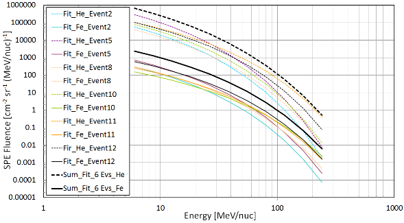
| Figure 10. Differential fluence energy spectra for protons, alpha particles, oxygen, magnesium , iron and summed spectra for Z>28 elements for a 2-year mission during solar maximum at the 90% confidence level. |
The energy range used for solar particle flux calculations is from 0.1 MeV/nucleon up to 500 MeV/nucleon. For geomagnetic shielding calculations all ions are treated as fully ionised.
| Event | A (cm-2s-1sr-1MeV-2) | κ | α |
|---|---|---|---|
| 19 Oct. 1989 | 214 | 0.526 | 0.366 |
| 22 Oct. 1989 | 429 | 0.458 | 0.3908 |
| 24 Oct. 1989 | 54900 | 2.38 | 0.23 |
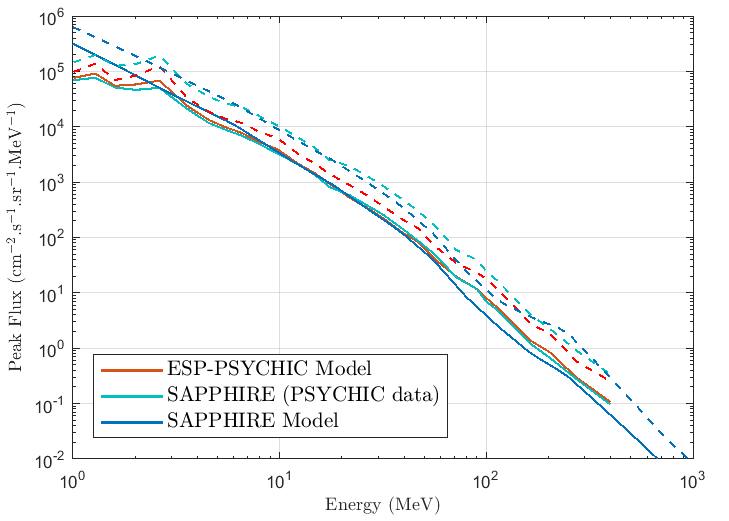
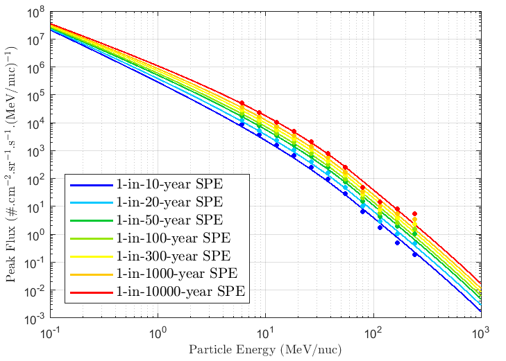
Similarly to the largest SPE fluence, results from SAPPHIRE can be transformed to provide outputs of 1-in-x-year SPE peak fluxes as a function of energy are given below:
As the geomagnetic cutoff varies with the particle's arrival direction, the geomagnetic cutoff transmission is averaged over all arrival directions. For a given location and rigidity, the integrated solid angle from where particles with this rigidity can reach the location, divided by 4pi, is called the attenuation or exposure factor. The attenuation factor for each proton energy is averaged over the spacecraft orbit and then multiplied with the interplanetary proton fluence provided by the proton models. For a given energy, the exposure time is defined as the total time that the orbit is in regions where the attenuation factor is non-zero. SPENVIS provides the attenuation for each orbital point and each proton energy, the orbit averaged attenuation factor, and the exposure time.
The presence of the solid Earth occults part of the solid angle from which particles can arrive at a given location. This effect is included in the calculation of the attenuation factor.
During magnetic storms, the geomagnetic cutoff is altered, usually allowing penetration to any given point in the magnetosphere by lower energy particles than is normally possible. A simple expression is used to account for this effect on the attenuation factor. Solar events are often, but not always, accompanied by magnetic storms at the Earth. Therefore, the user has the option of selecting a quiet or disturbed magnetosphere.
The calculation of the attenuation factor is based on a number of approximations that limit the validity of the result. It is well established that solar protons can penetrate much deeper in the magnetosphere than predicted by the simple attenuation model. Therefore, the user has the option of switching off the geomagnetic attenuation (this does not affect the Earth shadowing effect) to have an idea of the worst case effect of solar events.
Adams, J. H., Cosmic Ray Effects on Microelectronics, Part IV, NRL Memorandum Report 5901, Washington, D.C., 1986.
Asplund, M., Grevesse, N., Jacques Sauval, A., Scott, P., The chemical composition of the Sun, Annual Review of Astronomy & Astrophysics, Volume 47, Issue 1, pp. 481-522, 2009.
Burrell, M. O., The Risk of Solar Proton Events to Space Missions, NASA Report TMX-2440, 1972.
Crosby, N., Heynderickx, D., Jiggens, P., Aran, A., Sanahuja, B., Truscott, P., Lei, F., Jacobs, C., Poedts, S., Gabriel, S., Sandberg, I., Glover, A. & Hilgers, A., SEPEM: A tool for statistical modeling the solar energetic particle environment, Space Weather, 13(7), 2015.
Feynman, J., T. P. Armstrong, L. Dao-Gibner, and S. Silverman, New Interplanetary Proton Fluence Model, J. Spacecraft and Rockets, 27, 403, 1990.
Feynman, J., T. P. Armstrong, L. Dao-Gibner, and S. Silverman, Solar Proton Events During Solar Cycles 19, 20, and 21, Solar Phys., accepted November 1989.
Feynman, J., G. Spitale, J. Wang, and S. Gabriel, Interplanetary Proton Fluence Model: JPL 1991, J. Geophys. Res., 98, 13,281-13,294, 1993.
Feynman, J., A. Ruzmaikin, and V. Berdichevsky, The JPL proton fluence model: an update, JASTP, 64, 1679-1686, 2002.
Gabriel, S. B., and J. Feynman, Power-Law Distribution for Solar Energetic Proton Events, Sol. Phys., 165, 337-346, 1996.
Glover, A., Hilgers, A., Rosenqvist, L. and Bourdarie, S.: Interplanetary proton cumulated fluence model update, Advances in Space Research, Volume 42, Issue 9, 3 November 2008, Pages 1564-1568
Jiggens, P.T.A. & Gabriel, S.B., Time distributions of solar energetic particle events: Are SEPEs really random?, Journal of Geophysical Research, Volume 114(A10):A10105, 2009.
Jiggens, P., Gabriel, S.B., Heynderickx, D., Crosby, N., Glover, A. & Hilgers, A. ESA SEPEM Project: Peak Flux and Fluence Model, IEEE Transactions on Nuclear Science, Volume 59, Issue 4, 2012.
Jiggens, P., Varotsou, A., Truscott, P., Heynderickx, D., Lei, F., Evans, H. & Daly, E., The Solar Accumulated and Peak Proton and Heavy Ion Radiation Environment (SAPPHIRE) Model, IEEE Transactions on Nuclear Science, Volume 65, Issue 2, 2018a.
Jiggens, P., Heynderickx, D., Sandberg, I., Truscott, P., Raukunen, O. & Vainio, R., Updated Model of the Solar Energetic Proton Environment in Space, Journal of Space Weather and Space Climate, accepted manuscript, 2018b.
Kapur, J. N., Maximum Entropy Models in Science and Engineering, John Wiley & Sons, Inc., NY, 1989.
King, J. H., Solar Proton Fluences for 1977-1983 Space Missions, J. Spacecraft Rockets, 11, 401, 1974.
Lepreti, F., Carbone, V. & Veltri, P. Solar flare waiting time distribution: Varying rate-Poisson or Lèvy function? The Astrophysical Journal, Volume 555(L113-L136), 2001.
Nymmik, R.A., Improved environment radiation models. Advances in Space Research, 40(313-320), 2007.
Reames, D.V., Solar energetic particles: Sampling coronal abundances, Space Science Reviews, volume 85(1–2), pp. 327–340, 1998.
Rosenqvist, L., Hilgers, A., Evans, H., Daly, E.A., Hapgood, M., Stamper, R., Zwickl, R., Bourdarie, S. and Boscher, D., Toolkit for Updating Interplanetary Proton-Cumulated Fluence Models, Journal of Spacecraft and Rockets, Vol. 42, No. 6, 2005.
Sandberg, I., Jiggens, P., Heynderickx, D. & Daglis, I.A., Cross calibration of NOAA GOES solar proton detectors using corrected NASA IMP-8/GME data, Geophysical Research Letters, Volume 31, Issue 13, 2014.
Shea, M. A., D. F. Smart, J. H. Adams, D. Chenette, J. Feynman, D. C. Hamilton, G. Heckman, A. Konradi, M. A. Lee, D. S. Nachtwey, and E. C. Roelof, Toward a descriptive model of solar particles in the heliosphere, in Interplanetary Particle Environment, JPL Publication 88-28, 1988.
Smart, D. F., Predicting the Arrival Times of Solar Particles, in Interplanetary Particle Environment, JPL Publication 88-28, 1988.
Stassinopoulos, E. G., SOLPRO: A Computer Code to Calculate Probabilistic Energetic Solar Proton Fluences, NSSDC 75-11, Greenbelt, Maryland, 1975.
Tranquille, C., and E. J. Daly, An Evaluation of Solar-Proton Event Models for ESA Missions, ESA Journal, 16, 275-297, 1992.
Tylka, A.J., Dietrich, W.F. and Boberg, P.R., Probability Distributions of High-Energy Solar-Heavy-Ion Fluxes from IMP-8: 1973-1996, IEEE Trans. on Nucl. Sci., 44, 2140-2149 (1997)
Tylka, A. J., et al., CREME96: A Revision of the Cosmic Ray Effects on Micro-Electronics Code, IEEE Trans. Nucl. Sci., 44, 2150-2160, 1997a.
Tylka, A. J., Dietrich, W. F. and Boberg, P. R., Probability distributions of high-energy solar-heavy-ion fluxes from IMP-8: 1973-1996, IEEE Trans. Nucl. Sci., vol. 44, no. 6, pp. 2140–2149, Dec. 1997b.
Wheatland, M.S., The origin of the solar flare waiting-time distribution, The Astrophysical Journal, Volume 536(L109-L112), 2000.
M. Wheatland, The coronal mass ejection waiting-time distribution, Solar Physics, Volume 214, pp. 361-373, 2003.
Xapsos, M. A., G. P. Summers, and E. A. Burke, Extreme Value Analysis of Solar Energetic Proton Peak Fluxes, Solar Phys., 183, 157-164, 1998.
Xapsos, M. A., G. P. Summers, J. L. Barth, E. G. Stassinopoulos, and E. A. Burke, Probability Model for Worst Case Solar Proton Event Fluences, IEEE Trans. Nucl. Sci., 46, 1481-1485, 1999.
Xapsos, M. A., G. P. Summers, J. L. Barth, E. G. Stassinopoulos, and E. A. Burke, Probability Model for Cumulative Solar Proton Event Fluences, IEEE Trans. Nucl. Sci., 47, 486-490, 2000.
Xapsos, M.A., R J Walters, G P Summers, J L Barth, E G Stassinopoulos, S R Messenger, E A Burke, Characterizing solar proton energy spectra for ra-diation effects applications, IEEE Trans. on Nucl. Sci , 47, no. 6, pp 2218-2223, Dec. 2000.
Xapsos, M. A., Stauffer, C., Jordan, T., Barth, J.L., and Mewaldt, R.A., Model for Cumulative Solar Heavy Ion Energy and Linear Energy Transfer Spectra, IEEE Trans. On Nucl. Science, 54, No. 6, 2007.
Yucker, W. R., Solar Cosmic Ray Hazard to Interplanetary and Earth-Orbital Space Travel, NASA Report TMX-2440, 1972.