Spherical functions and their normalisations
Introduction
In geomagnetics, it is usual to describe the geomagnetic scalar potential
V as a series expansion of orthogonal spherical functions. These take
the form:
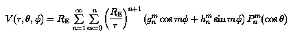
where RE is the mean radius of the Earth (6371.2 km),
r is the radial distance from the center of the Earth, phi is the
east longitude measured from Greenwich, theta is the geocentric
colatitude, and Pnm is the associated Legendre
function of degree n and order m. These associated Legendre functions can be
normalized, as is described in the following paragraphs.
The notation we use here for indicating the different normalisations are in
accordance with Chapman and Bartels, 1940.
Legendre functions Pn(x)
The Legendre functions are solutions of the following second degree
differential equation:
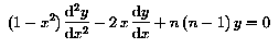
The general solution of this differential equation, disregarding the solutions
with n negative is given by:
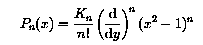
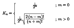
In this expression, the constant Kn is arbitrary. Usually,
the Legendre polynomial is normalized by imposing that Pn (1) = 1.
This results in the following expression:
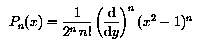
wich is called Rodrigues' formula for the Legendre polynomials.
Associated Legendre functions Pn,m(x)
The associated Legendre functions are the solutions of the associated
Legendre differential equation:
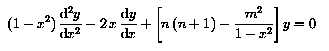
It is straightforward to verify that if y is a solution of the Legendre
differential equation, (1- x2)m/2
(d/dx)my is a solution of the associated
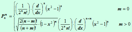
equation. We shall define, for positive integral m:
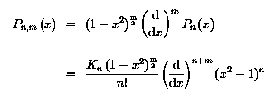
Pn,m is called an associated Legendre function. The second
solution of the differential equation, written Qn,m(x)
, is singular at x = 1 and -1 and will not concern us further.
The functions, used with the "normal" normalisation constant
Kn = 1/2n, were used by Neumann and Maxwell.
Gauss normalized associated Legendre functions
Pn,m (x)
Gauss and Laplace used functions with a Kn-value:
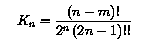
where in the notation (2n -1)!! = 1.3.5...(2n - 1) , as introduced by
Schuster by analogy with n!, and thus:
This is also the normalisation that is used in the model of
Jensen and Cain (1962).
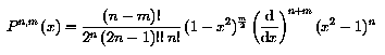
Schmidt quasi-normalized associated Legendre
functions Pnm(x)
Schmidt (1935) introduced the following
normalisation constant:
This makes the associated Legendre functions:
This form is used most in geomagnetic data, as it is the form which is used in
the International Geomagnetic Reference
Field (see
Peddie, 1982 and Langel, 1987). This normalisation
was introduced because it leaves the sum:
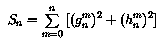
invariant under an arbitrary rotation of the (theta,phi) coordinate
system in the description of the scalar potential, and thus of the magnetic
field B.
Schmidt normalized associated Legendre functions Rnm(x)
The Schmidt quasi-normalized associated Legendre functions are not
completely normalized harmonics, in the sense that the average square value of
Pnm cos (m phi) or
Pnm sin (m phi) over the sphere is not equal
to 1. Schmidt introduced the functions:
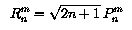
which are totally normalized. They were used for a time by Schuster, but were
given up later for use in geomagnetic models. However, they are in common use
in gravitational models.
References
Chapman, S. and Bartels, J., Geomagnetism, Oxford Un. Press Ed.,
pp. 609-612, 1940.
Jensen, D. C. and Cain, J. C., An interim geomagnetic field (abstract), J.
Geophys. Res., 67, pp. 3568-3569, 1962.
Langel, R. A., Main Field, Chapter Four in Geomagnetism, ed. J. A.
Jacobs, Academic Press, London, 1987.
Peddie, N. W., International Geomagnetic Reference Field: The Third
Generation, J. Geomag. Geoelectr., 34, pp. 309-326, 1985.
Schmidt, A., 1935.
Last update: Mon, 12 Mar 2018